Scene generation / Scene drawing
You can download the code blocks on this page as a notebook.
This tutorial describes the generation of synthetic images. Please make sure you’ve generated some cell simulation data from the Bacterial growth simulations part of these docs.
Synthetic mother machine images
The first thing we need to do is load in the important data we saved from the previous section. This includes the cell_timeseries_properties object (which defines each cell’s properties in every timepoint), and the main_segments object, which defines the trench geometry.
cell_timeseries_properties which we generated in Bacterial growth simulationsfrom SyMBac.PSF import get_condensers
from SyMBac.general_drawing import get_space_size, convolve_rescale
from joblib import Parallel, delayed
from tqdm.notebook import tqdm
from SyMBac.phase_contrast_drawing import draw_scene, generate_PC_OPL, make_images_same_shape, generate_training_data
from SyMBac.misc import get_sample_images
import pickle
import matplotlib.pyplot as plt
cell_timeseries_properties_file = open("cell_timeseries_properties.p", "rb")
cell_timeseries_properties = pickle.load(cell_timeseries_properties_file)
cell_timeseries_properties_file.close()
main_segments_file = open("main_segments.p", "rb")
main_segments = pickle.load(main_segments_file)
main_segments_file.close()
PSF generation
The next thing we must do is define the optical parameters which define the microscope simulation. You should know what phase contrast condensor you are using, you have the choice between the ‘Ph1’, ‘Ph2’, ‘Ph3’, ‘Ph4’, and ‘PhF’ condensors.
Note
If you only intend to generate fluorescence images, then you can choose any condenser key you want. It will not change the simulation.
W, R, diameter: The
get_condensers()function returns a dictionary of condensers for which you can pick a key from the above list. This will in turn return the dimensions of the chosen condenser.radius: The radius of the PSF convolution kernel to be generated. Must be an even number.
λ: The average wavelength of the illumination light source.
resize_amount: This is the “upscaling” factor for the simulation and the entire image generation process. Must be the same as the value defined in Running a simple simulation of cell growth in the mother machine.
pix_mic_conv: The number of microns per pixel. Again, should be the same value as defined in Running a simple simulation of cell growth in the mother machine..
NA: The numberical aperture of the objective lens.
n: The refractive index of the imaging medium.
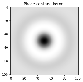
sigma and min_sigma: This is the sigma parameter for a 2D Gaussian which will be multiplied by the phase contrast kernel. This simulates apodisaton within the objective lens to attenuate halo and increase contrast. min_sigma is a calculated theoretical smallest Gaussian which would result in maximum apodisation. In reality the achieved apodisation is far from ideal.
## Fixed parameters given by the scope and camera
condensers = get_condensers()
W, R, diameter = condensers["Ph3"]
radius = 50 #I've found 50 to be the best kernel size to optimise convolution speed while maintaining accuracy
λ = 0.75
resize_amount = 3
pix_mic_conv = 0.0655 #0.108379937 micron/pix for 60x, 0.0655 for 100x
scale = pix_mic_conv / resize_amount
NA = 1.45
n = 1.4

## Free parameters given by the undefined apodisation of the objective.
## If unsure, leave this unchanged
min_sigma = 0.42*0.6/6 / scale #micron
sigma = min_sigma*10

kernel_params = (R,W,radius,scale,NA,n,sigma,λ) #Put into a tuple for easy use later
temp_kernel = get_phase_contrast_kernel(*kernel_params)
plt.imshow(temp_kernel, cmap="Greys_r")
plt.title("Phase contrast kernel")
Scene drawing
Now we can use the draw_scene() function to extract information from the simulation and redraw the cells as an image, applying transformations as necessary. We have some additional parameters which need specifying.
do_transformation: Whether or not to use each cell’s transformation attributes to bend or morph the cells to increase realism.
Warning
In extreme cases (very narrow trenches), setting this to do_transformation to True will cause clipping with the mother machine wall.
offset: This is a parameter which ensures that cells never touch the edge of the image after being transformed. In general this can be left as is (30), but you will recieve an error if it needs increasing.
label_masks: This controls whether the output training masks will be binary or labeled. Binary masks are used to train U-net, wheras labeled masks are used to train Omnipose
space_size: The size of the space used in the simulation, governing how large the image shall be. This is typically autocalculated using the
get_space_size()function.
After defining these arguments, we can pass them to draw_scene(), which will produce a list of scenes and corresponding masks for the entire simulation. Here we run this in parallel, for increased speed.
do_transformation = True
offset = 30
label_masks = True
space_size = get_space_size(cell_timeseries_properties)

scenes = Parallel(n_jobs=-1)(delayed(draw_scene)(
    cell_properties, do_transformation, space_size, offset, label_masks) for cell_properties in tqdm(cell_timeseries_properties, desc='Scene Draw:'))
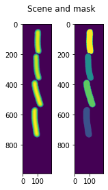
We can visualise what a scene (right) and its corresponding masks (right) look like. You can see that it is simply drawn as cells on a 0 background, with the intensity in each pixel corresponding to the thickness of the cell at that point. The masks are just the pixels where a cell can be found.
fig, (ax1, ax2) = plt.subplots(1, 2, figsize=(2.5,4))
fig.suptitle('Scene and mask')
ax1.imshow(scenes[-1][0])
ax2.imshow(scenes[-1][1])
plt.show()
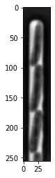
Now we need to load in a real image, this will be used to optimise the synthetic image. We provide real image samples in get_sample_images(). Here we use a 100x phase contrast image of E. coli.
Note
Ensure that the real image you load in is representative of the type of data you want to generate.
Ensure that you load in a real image as a NumPy array, and that it has even dimensions (otherwise you will get odd results if you try to fourier match).
real_image = get_sample_images()["E. coli 100x"]
print(real_image.shape)
plt.imshow(real_image,cmap="Greys_r")
plt.show()
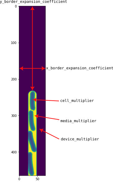
Next we will actually generate the fist truly synthetic image. We first generate a single sample, just to ensure we do not raise any errors, and to ensure that it is possible to generate a matching image given the chosen trench dimensions and real image dimensions. There are 5 parameters which need to be specified, described below and in the image below:
media_multiplier: The value to multiply the intensity of the media (area between cells and device)
cell_multiplier: The value to multiply the intensity of the cells’ pixels by.
device_multiplier: The value to multiply the device (PDMS) pixels by.
y_border_expansion_coefficient: A multiplier to fractionally scale the y dimension of the image by. Generally good to make this bigger than 1.5
x_border_expansion_coefficient: A multiplier to fractionally scale the x dimension of the image by.
Note
If the border_expansion_coefficient parameters are too small, you will be given an error asking you to increase their size. This may happen for any number of reasons, such as having a slightly too long trench in your simulation which just clips off the top of the image. Additionally, by expanding the borders of the image, we can more accurately convolve the PSF over the image withuot dealing with edge effects near the trench.
We now call a function called generate_PC_OPL(). This takes the above parameters, along with predefined offset, the scene and accompanying mask, along with two parameters, called defocus and fluorescence. The latter, when True, will simply switch off the trench and swap the phase contrast PSF for the fluorescence one. defocus as a numerical parameter which simulates out of focus effects in the image.
Note
It is not important to get any parameters perfect at this point, this is merely a test of whether the real image and synthetic image parameters are set correctly to enable generate_PC_OPL() to be called later to generate synthetic images with optimised parameters.
Finally we call convolve_rescale() from , which will convolve the kernel with the scene (with the expanded dimensions), at the upscaled resolution (the resize_amount argument), then resample it back down to the real image’s pixel size.
After this, make_images_same_shape() is called which will trim the expanded convolved image down to the same shape as the real image.
media_multiplier=30
cell_multiplier=1
device_multiplier=-50
y_border_expansion_coefficient = 1.9
x_border_expansion_coefficient = 1.4


temp_expanded_scene, temp_expanded_scene_no_cells, temp_expanded_mask = generate_PC_OPL(
main_segments=main_segments,
    offset=offset,
    scene = scenes[-3][0],
    mask = scenes[-3][0],
    media_multiplier=media_multiplier,
    cell_multiplier=cell_multiplier,
    device_multiplier=cell_multiplier,
    y_border_expansion_coefficient = y_border_expansion_coefficient,
    x_border_expansion_coefficient = x_border_expansion_coefficient,
    fluorescence=False,
    defocus=30
)


### Generate temporary image to make same shape

convolved = convolve_rescale(temp_expanded_scene, temp_kernel, 1/resize_amount, rescale_int = True)
real_resize, expanded_resized = make_images_same_shape(real_image,convolved, rescale_int=True)
Next we shall extract some pixels from the real image which we will use to optimise the synthetic image. We will extract the pixel intensities and variances from the 3 important regions of the image. The cells, the device, and the media. These are the same three aforementioned intensities for which we “guessed” some parameters in the previous code block.
We use napari to load the real image, and create three layers above it, called media_label, cell_label, and device_label. We will then select each layer and draw over the relevant regions of the image.
Note
You do not need to completely draw over all the cells, the entire device, or all the media gaps between the cells. Simply getting a representative sample of pixels is generally enough. See the video below for a visual demonstration.
import napari

viewer = napari.view_image(real_resize)
media_label = viewer.add_labels(np.zeros(real_resize.shape).astype(int), name = "media")
cell_label = viewer.add_labels(np.zeros(real_resize.shape).astype(int), name = "cell")
device_label = viewer.add_labels(np.zeros(real_resize.shape).astype(int), name = "device")
We then collate the output of this annotation into the means and variances of each individual image component, and we can subsequently save the information to a pickle so we don’t need to redraw on the image every time we want to run the code.
real_media_mean = real_resize[np.where(media_label.data)].mean()
real_cell_mean = real_resize[np.where(cell_label.data)].mean()
real_device_mean = real_resize[np.where(device_label.data)].mean()
real_means = np.array((real_media_mean, real_cell_mean, real_device_mean))

real_media_var = real_resize[np.where(media_label.data)].var()
real_cell_var = real_resize[np.where(cell_label.data)].var()
real_device_var = real_resize[np.where(device_label.data)].var()
real_vars = np.array((real_media_var, real_cell_var, real_device_var))

image_params = (real_media_mean, real_cell_mean, real_device_mean, real_means, real_media_var, real_cell_var, real_device_var, real_vars)

import pickle
image_params_file = open('image_params.p', 'wb')
pickle.dump(image_params, image_params_file)
image_params_file.close()

## For opening pregenerated image parameters
#image_params_file = open("image_params.p", "rb")
#image_params = pickle.load(image_params_file)
#image_params_file.close()
Finally, we will use the manual optimiser to generate a realistic image. The output from the optimiser will then be used to generate an entire dataset of synthetic images. Below the code is a video demonstrating the optimisation process.
from SyMBac.optimisation import manual_optimise

params = manual_optimise(
    scenes = scenes,
    scale = scale,
    offset = offset,
    main_segments = main_segments,
    kernel_params = kernel_params,
    min_sigma = min_sigma,
    resize_amount = resize_amount,
    real_image = real_image,
    image_params = image_params,
    x_border_expansion_coefficient = x_border_expansion_coefficient,
    y_border_expansion_coefficient = y_border_expansion_coefficient
)

params # Ensure you actually call the params object like this.
Finally, we generate our training data using generate_training_data(). The important parameters to recognise are:
sample_amount: This is a percentage by which all continuous parameters
manual_optimise()can be randomly scaled during the synthesis process. For example, a value of 0.05 will randomly scale all continuous parameters by \(X \sim U(0.95, 1.05)\) Higher values will generate more variety in the training data (but too high values may result in unrealistic images).randomise_hist_match: Whether to randomise the switching on and off of histogram matching.
randomise_noise_match: Whether to randomise the switching on and off of noise matching.
sim_length: The length of the simulation
burn_in: The number of frames at the beginning of the simulation to ignore. Useful if you do not want images of single cells to appear in your training data.
n_samples: The number of random training samples to generate.
save_dir: The save directory of the images. Will output two folders,
convolutionsandmasks.in_series: Whether or not to shuffle the simulation while generating training samples.
Note
When running generate_training_data(), you may choose to set in_series=True. This will generate training data whereby each image is taken sequentially from the simulation. This useful if you want train a tracking model, where you need the frames to be in order. If you choose to set in_series=True, then it is a good idea to choose a low value of sample_amount, typically less than 0.05 is sensible. This reduces the frame-to-frame variability.
generate_training_data(
    interactive_output = params,
    sample_amount = 0.05,
    randomise_hist_match = False,
    randomise_noise_match = True,
    sim_length = 1000,
    burn_in = 100,
    n_samples =  300,
    save_dir = "/tmp/",
    in_series=False
)