Mother machine simulations

%load_ext autoreload
%autoreload 2

import sys
sys.path.insert(1, '/home/georgeos/Documents/GitHub/SyMBac/') # Not needed if you installed SyMBac using pip

from SyMBac.simulation import Simulation
from SyMBac.PSF import PSF_generator
from SyMBac.renderer import Renderer
from SyMBac.PSF import Camera
from SyMBac.misc import get_sample_images
real_image = get_sample_images()["E. coli 100x"]

/home/georgeos/Documents/GitHub/SyMBac/SyMBac/cell_simulation.py:10: TqdmExperimentalWarning: Using `tqdm.autonotebook.tqdm` in notebook mode. Use `tqdm.tqdm` instead to force console mode (e.g. in jupyter console)
  from tqdm.autonotebook import tqdm
TiffPage 0: TypeError: read_bytes() missing 3 required positional arguments: 'dtype', 'count', and 'offsetsize'

Running a simulation

Mother machine simulations are handled with the Simulation class.

Instantiating a Simulation object requires the following arguments to be specified:

• trench_length: The length of the trench.

• trench_width: The width of the trench.

• cell_max_length: The maximum allowable length of a cell in the simulation.

• cell_width: The average width of cells in the simulation.

• sim_length: The number of timesteps to run the simulation for.

• pix_mic_conv: The number of microns per pixel in the simulation.

• gravity: The strength of the arbitrary gravity force in the simulations.

• phys_iters: The number of iterations of the rigid body physics solver to run each timestep. Note that this affects how gravity works in the simulation, as gravity is applied every physics iteration, higher values of phys_iters will result in more gravity if it is turned on.

• max_length_var: The variance applied to the normal distribution which has mean cell_max_length, from which maximum cell lengths are sampled.

• width_var: The variance applied to the normal distribution of cell widths which has mean cell_width.

• save_dir: The save location of the return value of the function. The output will be pickled and saved here, so that the simulation can be reloaded later withuot having to rerun it, for reproducibility. If you don’t want to save it, just leave it as /tmp/`.

More details about this class can be found at the API reference: SyMBac.simulation.Simulation()

my_simulation = Simulation(
    trench_length=15,
    trench_width=1.3,
    cell_max_length=6.65, #6, long cells # 1.65 short cells
    cell_width= 1, #1 long cells # 0.95 short cells
    sim_length = 100,
    pix_mic_conv = 0.065,
    gravity=0,
    phys_iters=15,
    max_length_var = 0.,
    width_var = 0.,
    lysis_p = 0.,
    save_dir="/tmp/",
    resize_amount = 3
)

We can then run the simulation by calling the SyMBac.simulation.Simulation.run_simulation() method on our instantiated object. Setting show_window=True will bring up a pyglet window, allowing you to watch the simulation in real time. If you run SyMBac headless, then keep this setting set to False, you will be able to visualise the simulation in the next step.

my_simulation.run_simulation(show_window=False)

Next we call SyMBac.simulation.Simulation.draw_simulation_OPL(), which will convert the output of the simulation to a tuple of two arrays, the first being the optical path length (OPL) images, and the second being the masks.

This method takes two arguments.

• do_transformation - Whether or not to bend or morph the cells to increase realism.

• label_masks - This controls whether the output training masks will be binary or labeled. Binary masks are used to train U-net (e.g DeLTA), wheras labeled masks are used to train Omnipose

my_simulation.draw_simulation_OPL(do_transformation=True, label_masks=True)

Simulation visualisation

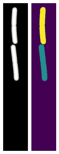
We can visualise one of the OPL images and masks from the simulation:

import matplotlib.pyplot as plt
fig, (ax1, ax2) = plt.subplots(1, 2, figsize=(2,5))
ax1.imshow(my_simulation.OPL_scenes[-1], cmap="Greys_r")
ax1.axis("off")
ax2.imshow(my_simulation.masks[-1])
ax2.axis("off")
plt.tight_layout()

Alternatively we can bring up a napari window to visualise the simulation interactively using SyMBac.simulation.Simulation.visualise_in_napari()

my_simulation.visualise_in_napari()

Point spread function (PSF) generation

The next thing we must do is define the optical parameters which define the microscope simulation. To do this we instantiate a PSF_generator, which will create our point spread functions for us. We do this by passing in the parameters defined in SyMBac.PSF.PSF_generator but below we show 3 examples:

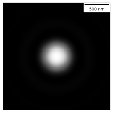
# A 2D simple fluorescence kernel based on Airy
my_kernel = PSF_generator(
    radius = 50,
    wavelength = 0.75,
    NA = 1.2,
    n = 1.3,
    resize_amount = 3,
    pix_mic_conv = 0.065,
    apo_sigma = None,
    mode="simple fluo")
my_kernel.calculate_PSF()
my_kernel.plot_PSF()

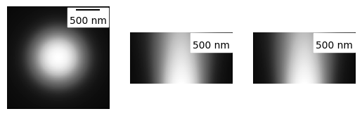
# A 3D fluorescence kernel based on the psfmodels library
# (note the larger looking PSF due to the summed projection)
# (During convolution, each slice of the image is convolved with the relevent
# volume slice of the cell)
my_kernel = PSF_generator(
    z_height=50,
    radius = 50,
    wavelength = 0.75,
    NA = 1.2,
    n = 1.3,
    resize_amount = 3,
    pix_mic_conv = 0.065,
    apo_sigma = None,
    mode="3D fluo")
my_kernel.calculate_PSF()
my_kernel.plot_PSF()

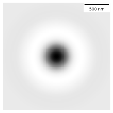
# A phase contrast kernel
my_kernel = PSF_generator(
    radius = 50,
    wavelength = 0.75,
    NA = 1.2,
    n = 1.3,
    resize_amount = 3,
    pix_mic_conv = 0.065,
    apo_sigma = 20,
    mode="phase contrast",
    condenser = "Ph3")
my_kernel.calculate_PSF()
my_kernel.plot_PSF()

Camera model

Next we optionally define a camera based on SyMBac.camera.Camera(), if your camera properties are known. If you do not know them, then you will be allowed to do ad-hoc noise matching during image optimisation.

my_camera = Camera(baseline=100, sensitivity=2.9, dark_noise=8)
my_camera.render_dark_image(size=(300,300));

Rendering

Next we will create a renderer with SyMBac.renderer.Renderer(), this will take our simulation, our PSF (in this case phase contrast), a real image, and optionally our camera.

my_renderer = Renderer(simulation = my_simulation, PSF = my_kernel, real_image = real_image, camera = my_camera)

Next we shall extract some pixels from the real image which we will use to optimise the synthetic image. We will extract the pixel intensities and variances from the 3 important regions of the image. The cells, the device, and the media. These are the same three aforementioned intensities for which we “guessed” some parameters in the previous code block.

We use napari to load the real image, and create three layers above it, called media_label, cell_label, and device_label. We will then select each layer and draw over the relevant regions of the image.

A video below shows how it’s done:

Note

You do not need to completely draw over all the cells, the entire device, or all the media gaps between the cells. Simply getting a representative sample of pixels is generally enough. See the video below for a visual demonstration.

from IPython.display import YouTubeVideo
YouTubeVideo("sPC3nV_5DfM")

my_renderer.select_intensity_napari()

Finally, we will use the manual optimiser (SyMBac.renderer.Renderer.optimise_synth_image()) to generate a realistic image. The output from the optimiser will then be used to generate an entire dataset of synthetic images. Below the code is a video demonstrating the optimisation process.

YouTubeVideo("PeeyotMQAQU")

my_renderer.optimise_synth_image(manual_update=False)

Finally, we generate our training data using SyMBac.renderer.Renderer.generate_training_data().

The important parameters to recognise are:

• sample_amount: This is a percentage by which all continuous parameters manual_optimise() can be randomly scaled during the synthesis process. For example, a value of 0.05 will randomly scale all continuous parameters by \(X \sim U(0.95, 1.05)\) Higher values will generate more variety in the training data (but too high values may result in unrealistic images).

• randomise_hist_match: Whether to randomise the switching on and off of histogram matching.

• randomise_noise_match: Whether to randomise the switching on and off of noise matching.

• sim_length: The length of the simulation

• burn_in: The number of frames at the beginning of the simulation to ignore. Useful if you do not want images of single cells to appear in your training data.

• n_samples: The number of random training samples to generate.

• save_dir: The save directory of the images. Will output two folders, convolutions and masks.

• in_series: Whether or not to shuffle the simulation while generating training samples.

Note

When running this, you may choose to set in_series=True. This will generate training data whereby each image is taken sequentially from the simulation. This useful if you want train a tracking model, where you need the frames to be in order. If you choose to set in_series=True, then it is a good idea to choose a low value of sample_amount, typically less than 0.05 is sensible. This reduces the frame-to-frame variability.

my_renderer.generate_training_data(sample_amount=0.1, randomise_hist_match=True, randomise_noise_match=True, burn_in=40, n_samples = 500, save_dir="/tmp/test/", in_series=False)

Sample generation: 100%|██████████████████████| 500/500 [00:50<00:00,  9.81it/s]